What is Structured Meshing?

Introduction
Structured meshing is a foundational technique in computational simulations, especially in fields like computational fluid dynamics (CFD), heat transfer, and structural mechanics. At its core, it involves dividing a physical domain into a logically ordered arrangement of smaller elements or cells that serve as the basis for numerical analysis. Each of these cells represents a control volume in which governing physical laws are applied.
What distinguishes structured meshing from other approaches is its regularity. Cells are arranged in a grid where their positions and neighbors are known simply by their location within an indexing system. This level of predictability not only facilitates efficient storage and processing but also leads to faster and more accurate simulations. As simulation problems grow more complex, structured meshing continues to evolve, incorporating sophisticated strategies like multi-block partitioning and overset methodologies to handle challenging geometries without compromising on computational efficiency.
What is a Structured Mesh?
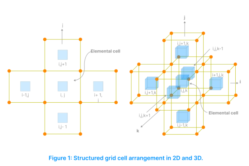
A structured mesh is a grid in which elements are organized in a regular, topologically consistent pattern. In two-dimensional problems, this typically results in quadrilateral cells, while in three-dimensional domains, the grid is composed of hexahedral cells. Each cell is associated with a set of integer indices, often denoted as (i, j, k), which uniquely identify its location within the mesh and allow direct access to neighboring elements by simple arithmetic on the indices.
This structured arrangement simplifies many aspects of numerical computation. For instance, accessing a neighboring cell requires nothing more than incrementing or decrementing an index. Because of this implicit connectivity, there is no need to store complex data structures to manage relationships between cells, leading to efficient memory usage. Furthermore, the regularity of the mesh makes it easier to implement solvers, simplifies debugging, and supports high-performance parallel computing.
In practical simulations, each cell in a structured mesh serves as a control volume where conservation laws of mass, momentum, energy, and other physical quantities are applied. The precision with which these laws are enforced often depends on the quality of the mesh, which makes the structured approach particularly appealing when accuracy and computational speed are critical.
Types of Structured Grids
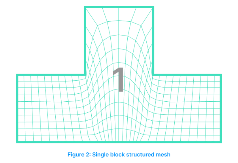
Single-Block Structured Grids
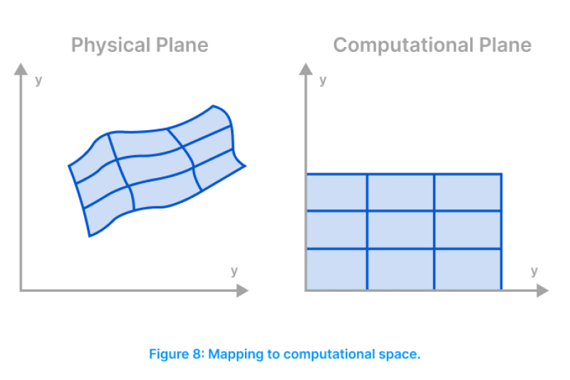
Single-block grids represent the simplest form of structured meshing. In this approach, the entire computational domain is covered using one continuous, logically rectangular block of cells. The domain is typically mapped into a unit square or cube in computational space, where grid points are distributed using algebraic functions or by solving governing equations in a transformed coordinate system.
Although the single-block method offers simplicity and ease of implementation, it has severe limitations when applied to complex geometries. When trying to conform a single grid block to curved or irregular boundaries, cells may become highly stretched, skewed, or folded. These geometric distortions can negatively impact the accuracy of simulations and lead to convergence difficulties.
Single-block grids also offer little flexibility in refining specific regions of interest within the domain. Since the grid structure is continuous and uniform, refining the mesh in one area often leads to unnecessary refinement elsewhere, thereby increasing computational cost without corresponding benefits in accuracy. Despite these drawbacks, single-block grids are still used for simple geometries where such limitations are minimal.
Block-Structured Grids (Multi-Block)
Block-structured grids provide a more flexible and powerful alternative to single-block grids. In this strategy, the domain is divided into multiple structured blocks that are meshed individually. Each block maintains its own structured topology, but the combination of blocks allows the mesh to conform to complex geometrical features.

The use of multiple blocks introduces a level of adaptability that is crucial for accurately representing intricate surfaces, edges, and corners. It also allows for localized mesh refinement. For example, blocks can be made finer in regions where flow gradients are steep, such as boundary layers or shock fronts, while keeping coarser grids in areas of relatively uniform flow. This selective refinement optimizes both accuracy and computational efficiency.
Another advantage of block-structured grids is their ability to produce high-quality cells throughout the domain. By aligning blocks with the natural geometry of the object being simulated, mesh skewness and cell distortion can be significantly reduced. This leads to smoother grids that improve the numerical properties of the simulation, enhancing both stability and convergence.
Multi-Block Connectivity: Interface Types
Conformal vs Non-Conformal Interfaces
The manner in which adjacent blocks connect to each other plays a significant role in mesh quality and solver performance. In a conformal interface, the faces of neighboring blocks align perfectly. Grid nodes at the shared interface match exactly, allowing flow variables to be passed directly between blocks without the need for interpolation.
Conformal interfaces are desirable because they are easy to implement numerically and help maintain the conservation of physical quantities across block boundaries. However, achieving conformal connectivity in complex geometries often requires considerable effort. It may necessitate aligning resolutions and orientations across multiple blocks, which can complicate the meshing process.


Non-conformal interfaces, on the other hand, allow the adjacent blocks to have mismatched nodes and faces at their common boundaries. This added flexibility makes it easier to construct grids for intricate geometries. Blocks can be independently designed with resolutions and shapes that best suit their local regions. To maintain continuity during simulation, interpolation schemes are employed to exchange information between non-matching interfaces.
Although interpolation introduces a minor increase in computational effort and the potential for slight numerical diffusion, the benefits in terms of mesh flexibility and quality often outweigh these drawbacks. Non-conformal connectivity is particularly useful when implementing advanced blocking strategies such as C-type or O-type topologies that better capture flow features like separation or circulation.
Full vs Partial Matching Interfaces
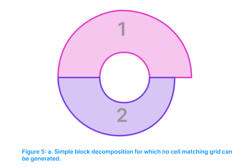
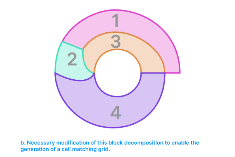
Block interfaces can also be classified based on the extent to which they share common boundaries. In full matching interfaces, the adjacent blocks align perfectly across their shared face. Every node and edge on one side corresponds to a node and edge on the other. This type of interface ensures continuity and simplifies numerical handling.
However, creating full matching interfaces often demands a higher number of blocks, particularly in geometries with irregular shapes or abrupt transitions. As a result, block management and visualization can become more complex.
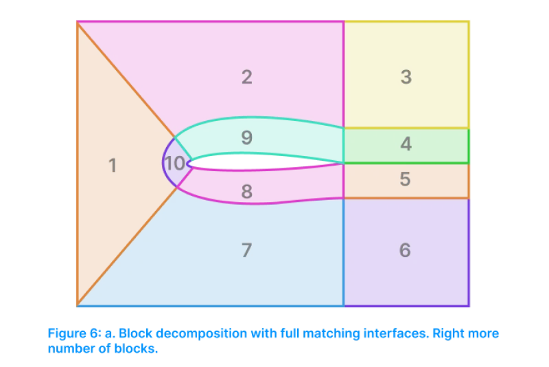
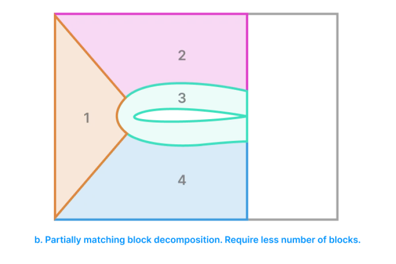
Partial matching interfaces, by contrast, allow only a portion of one block’s face to coincide with a portion of its neighbor’s face. This partial overlap provides greater flexibility in block construction and enables the use of fewer blocks to achieve the same geometric fidelity. In practice, simulation tools often support such configurations by implementing interpolation routines that bridge the interface.
In structured meshing software such as GridPro, fully matched blocks are referred to as elementary blocks. When multiple elementary blocks are merged into a single logical unit, the result is known as a super-block. Super-blocks simplify visualization and reduce the overall block count, making them a valuable concept in managing large-scale simulations.
Overset (Chimera) Grids
Overset grids, also known as Chimera grids, represent a special case where blocks are allowed to overlap. Instead of connecting through shared interfaces, each block is generated independently and is positioned to overlap with one or more other blocks. Interpolation is then used to transfer information between overlapping regions.
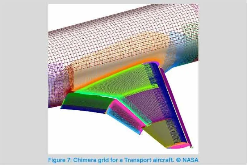
This approach is especially useful when meshing highly complex assemblies or components in motion. For instance, rotating blades or moving control surfaces can be meshed as separate blocks and moved independently during the simulation. Overset grids eliminate the need for deforming or remeshing the entire domain, which simplifies both setup and computation.
Despite their flexibility, overset grids introduce additional complexity in terms of interpolation accuracy and data management. Careful attention must be paid to ensure that overlapping regions are handled correctly and that conservation of physical quantities is maintained. Nonetheless, their benefits in handling dynamic and composite geometries have made them a popular choice in advanced simulations.
Structured Grid Generation Techniques
Generating a high-quality structured mesh involves determining the positions of grid points in a way that captures the geometry accurately and supports robust computation. The two primary approaches to grid generation are algebraic methods and techniques based on solving partial differential equations.
Algebraic Method (Transfinite Interpolation - TFI)
The algebraic approach to grid generation is based on direct interpolation between boundary points. In the widely used transfinite interpolation method, the physical domain is mapped to a computational domain, such as a square or cube. Using mathematical blending functions, interior grid points are computed based on the known locations of boundary nodes.
This method is extremely fast and simple to implement. It offers explicit control over grid spacing and point distribution, making it suitable for applications where quick results are needed. Grid clustering near surfaces or within regions of interest can be achieved by manipulating interpolation parameters.
However, algebraic methods do have limitations. They provide little control over grid smoothness and are prone to generating skewed or distorted cells in complex geometries. Discontinuities at boundaries can easily propagate into the interior, reducing overall mesh quality. As such, algebraic methods are often used in combination with smoothing techniques or as a first step before more refined generation using PDE methods.
PDE-Based Methods
In contrast to algebraic techniques, PDE-based methods generate grids by solving partial differential equations that govern the distribution and alignment of grid lines. These methods provide higher quality meshes and greater control over cell size, shape, and orientation.
In the elliptic PDE method, a system of Poisson equations is solved iteratively. Control functions, also called source terms, are introduced to influence grid characteristics such as orthogonality, clustering, and smoothness. This approach is particularly effective in producing smoothly varying grids with good alignment to physical boundaries. However, it is computationally expensive and may require considerable tuning of control parameters.
Hyperbolic PDE methods offer an alternative strategy that is particularly effective for external flow problems. Here, the grid is generated in a marching fashion, beginning from a known boundary and propagating outward. This results in fast computation and naturally orthogonal grids, though the method is sensitive to boundary discontinuities and cannot be applied easily to closed domains.
Each of these PDE-based methods has its own strengths and limitations. Elliptic methods are best for high-quality grids in confined geometries, while hyperbolic methods are preferred for rapid grid generation in open domains.
Conclusion
Structured meshing continues to serve as a fundamental technique in numerical simulations, offering unmatched efficiency and accuracy in many applications. From its simplest form in single-block grids to the highly adaptable multi-block and overset configurations, structured meshing provides a versatile and powerful approach for tackling a wide variety of engineering problems.
Though it may demand careful planning and manual effort, the rewards in terms of simulation performance are significant. With advancements in meshing software and automation, the barriers to using structured grids are gradually being lowered, making it accessible to a broader range of users.
In simulations where precision and performance are paramount, structured meshing remains not just relevant but indispensable.